Page 10 / 20
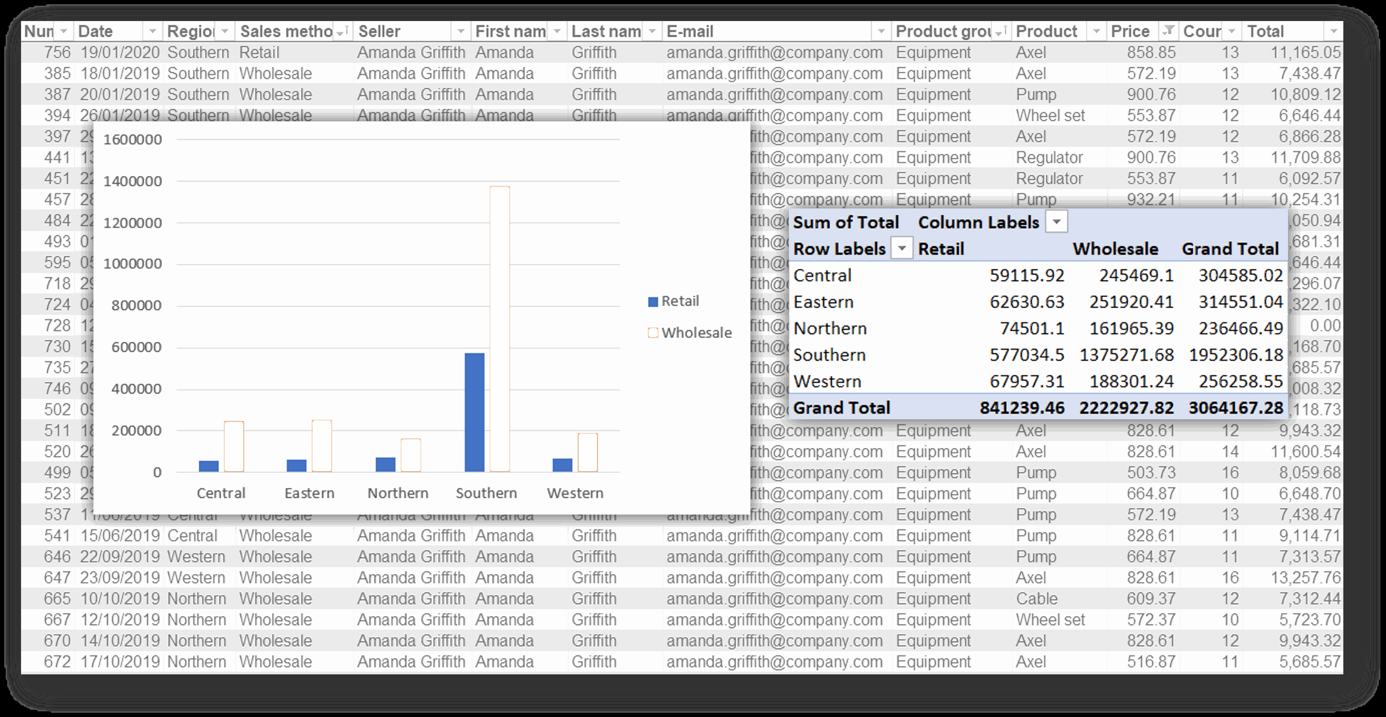
Pivot tables are a tool for quick summaries of data. The summaries generated by the pivot tables can also be easily visualised as a chart.
Below is an example of a pivot report with both a pivot table and an associated chart. It is easy to understand what the report describes, and it is rather clear. It won't take you a minute to write this report, and by the end of this chapter you'll be able to do it.
Kuva pivot-raportoinnista. Note
### A message from a student
The pivot table has always been such a boogeyman for me. I have never been able to get them right. Now that I was able to get hands-on help with them, I realized that they were not as impossible as I had previously thought.
Now I dare to take them on and try them out. This is very useful when you need to work on reporting.
Heidi Niinimäki , City of Tampere
Source material
A pivot table can be created from data on an Excel sheet, or it can be created from an external data source. In this training, we will create pivot tables from the data we have already worked with.
It is recommended that the source material is converted into a table to ensure the correct structure. If more rows or columns are added to the data, they can then be easily updated in pivot tables.
The first row of the source material table must contain the column header in each column, and there must be no blank rows or columns. If the data has not been converted into a table, there must be a blank line between the calculation rows and the actual data.
A pivot table has been added to the Sales by region spreadsheet. In the pivot table we have Sales method as a column, Region and Product group as rows and Grand Total as values. Model:
Task: Create a new pivot table
Let's start by creating a new pivot table to summarize the Sales table we have worked on.
Nice
Creating a pivot table
Select a table by clicking on one of its cells.
Create a pivot table by clicking on the **Summarize with PivotTable ** button in the **Tools ** group on the **Table Design ** in tab.
Luo Pivot‑taulukko -ikkuna In the window that opens, you can further configure the settings of the new pivot table. Check that the data source is indeed the Sales table and that the pivot table is created on a new sheet (select New Worksheet OK .
Näkymä, kun pivot on valittu The pivot table was created on a new sheet, in this example Sheet1
When a cell is selected in the pivot area, two new tabs appear at the end of the selection ribbon: PivotTable Analyze Design
In addition, a field list opens in the right-hand side of the window, through which the pivot table will be built.
Question: Where can I get the list of fields visible again?
Sometimes the field list disappears (you have clicked the close button in its corner) and it no longer appears with the pivot table. In practice, you have closed it separately.
Nice
Displaying the field list
Kenttäluettelon lisääminen näytölle You can display the list again via the Field List Show PivotTable Analyze
Task: Add columns, rows and values to the pivot table
In the pivot we created, we add Sales method as a column, Region and Product group as rows and Sum of Total as value. Model:
Kuva mallitaulukosta Here's another example of a field list:
Suodattimet, sarakkeet, rivit ja arvot, joista suodattimet-kohdassa ei ole mitään Nice
## Putting fields into areas
Fields can be added to the pivot table in different ways, but one convenient way is as follows: Use your mouse to drag the field name in the list at PivotTable Fields Filters , Columns , Rows or Values ). The figure below illustrates how the different placements affect the different areas.
Rows
Columns
Values
Fields can also be dragged from one area to another, and a field can be deleted by dragging it outside the **PivotTable Fields ** area or by clicking the selection off the screen next to the field.
Task: Name the sheet “Sales by region”
Model:
Kaksi välilehteä, joista oikeanpuoleisin on Myynnit alueittain Nice
Double-click on the sheet selector and type a new name.
Are you ready?