Summaries in a Table
Tables provide a quick way to calculate column summaries. In practice, we can add a summary row below the table, called Total Row. Excel automatically calculates the summaries requested. The summary line differs from the usual formula in that it reacts to filtering of the table. (We'll deal with filtering in a moment.)
The most typical summaries are counting the number of rows (Count), the sum of rows (Sum) and the average of rows (Average).
The Objective
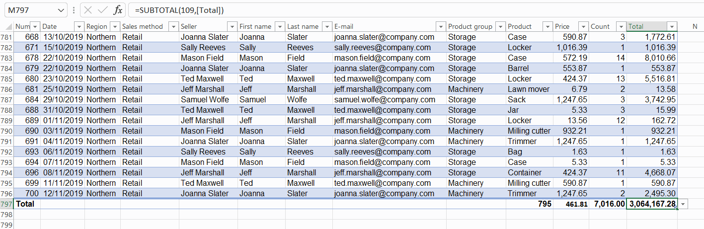
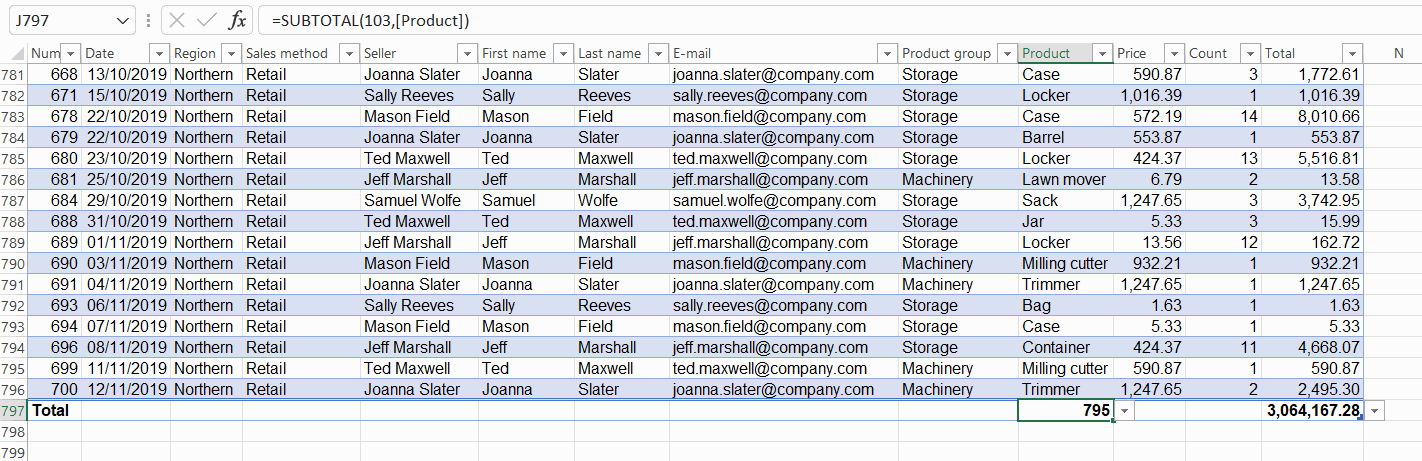
The table has the added Total Row, which calculates
- number of rows visible under the Product column
- Price column average
- Total number of products sold, i.e. the sum of the Count column
- Total sales, i.e. the sum of the Total column
Model:
Task: Add Total Row
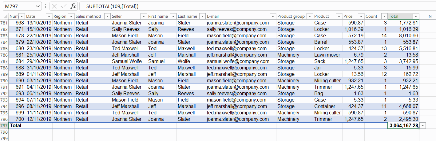
Info: A different formula
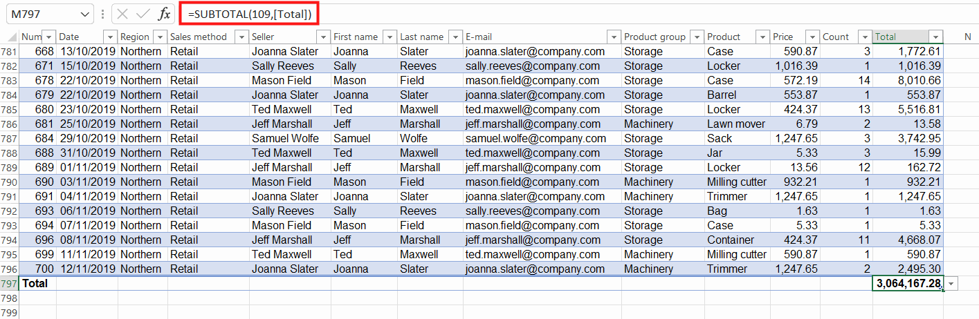
 | The summary formulas added as described above differ from the normal **SUM** and **COUNT** functions in that they react to the filtering of the table. If you look at the formula line, you'll see the **SUBTOTAL** function. |
This means that the formulas react to the filtering of the table: When hiding rows by filtering, Total Row will update with the changes.
Info: Modify or delete the summary
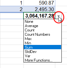
When you click on the summary cell, you will notice that a small triangle appears at the edge of the cell. You can change the formula to be calculated or remove it from the cell by clicking on the triangle.
Total Row can be configured to include other information. By clicking on any of its cells, you can add a formula of your choice, for example the average, under the column of your choice.
Task: Add the number of rows to the summary
Task: Add the average of prices
Add in the same way the Average summary to the Price column.
Task: Add the number of products sold
Add in the same way the Sum summary to the Count column.
Task: Change the title to “Total sales”
Let's change the header on the left side of the summary line. Let the title be “Total sales”.
Are you ready?