Formatting a Pivot Table

In a pivot table (as in Excel in general), you can format the appearance of cells in many ways. The main formatting aspects of the table are the coloring used, the number formats of the figures and the different options to add subtotals and blank lines to make the table clearer.

The Objective

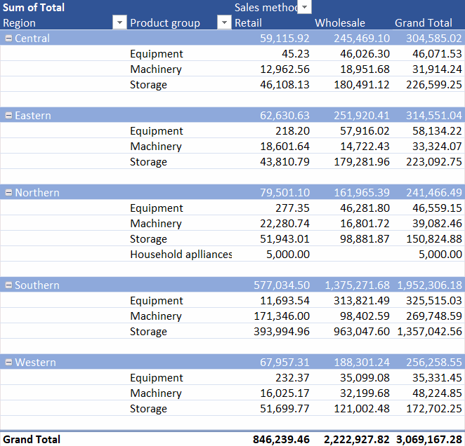
The pivot table has been formatted: Its color scheme has been slightly sharpened, thousands separators have been enabled in the number formats, the layout of the pivot table has been changed to structured, blank rows have been added between groups and subtotals have been moved to their own rows at the bottom of the groups. Model:

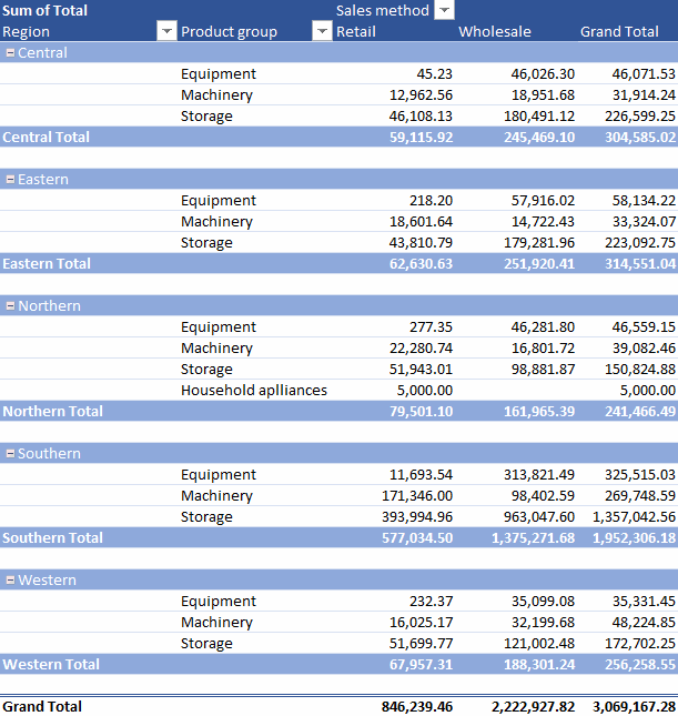
Task: Change the color scheme to a sharper blue

Change the color scheme to a sharper blue to make the headers between the lines stand out more clearly. Model:

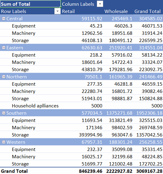
Task: Format all numbers using number formats

Now the figures in the pivot table have different shapes and are a bit difficult to perceive. Let's format them to use number formats with thousands separators.

Model:

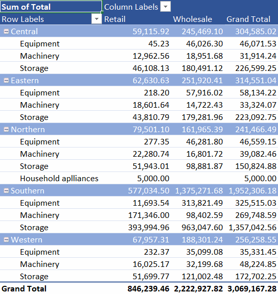
Task: Change the layout to outline view

Pivot tables support three different layouts: Show in Compact Form, Show in Outline Form and Show in Tabular Form. The default layout is Show in Compact Form. Change it to use the layout Show in Outline Form.

Model:

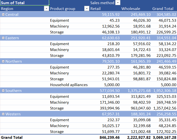
Task: Add blank rows

The pivot table can be made a little clearer by inserting blank rows between the groups. Model:

Task: Move the subtotals to the bottom of row group

Let's position the subtotals associated with the groups in the pivot table. Now they are placed up in the same row as the header. Let's move them down to their own rows.

Model:

Now the visual appearance of the pivot table has changed significantly. With these layouts, you'll find a clear presentation of your data, highlighting the right things. Next, we will look in more detail at the different summaries in the pivot table. Are you ready?