Subtotals and Summaries in a Pivot Table

The pivot table we have worked with so far shows the value of the desired field in each cell and the subtotals in the subtitles. However, we can modify these values. Excel offers a wide range of options for editing these.

The key concepts are:

• Summary type, i.e. what is shown in each cell. By default, the cell displays the sum, but you can display, for example, the number of rows in the data (Count) or the average.

• Format of values: This can be used to modify the way the value is presented. In particular, we can, for example, express the value as a percentage of the desired total.

• Subtitle: There can be several subtitles, and values can be calculated for them in a similar way to the value summary criteria.

The Objective

Sales by region has been modified to deal with the number of sales transactions, which are presented as a percentage of the row total. Model:

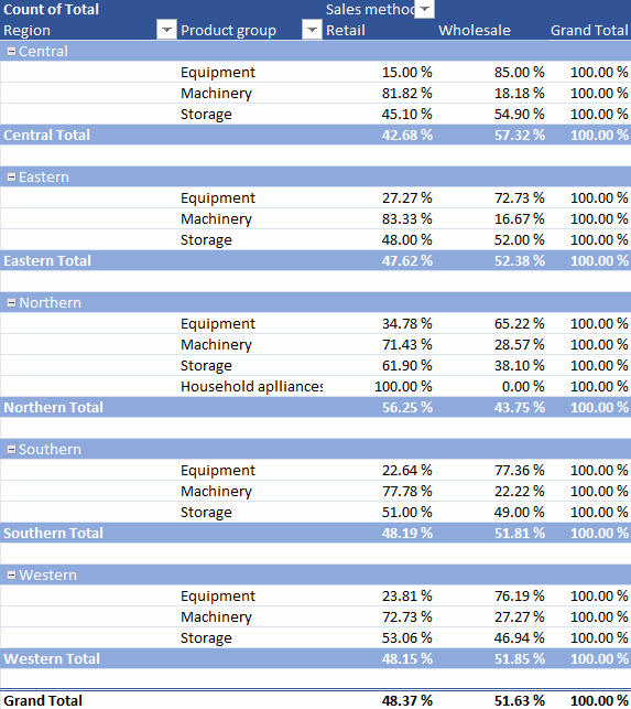
Task: Change the summary type to Count

Change the summary type to **Count** to see the number of transactions that have taken place. Model:

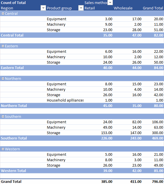
Task: Show values in the format “% of Row Total”

Show the values in the format % of Row Total, allowing you to compare by region and by product the number of wholesale and retail sales transactions. Model:

The Objective

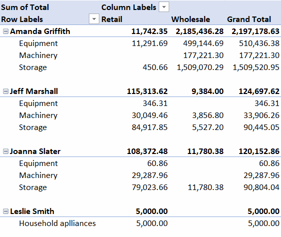
A Sales by seller pivot table has been added to the workbook, with Sales method as a column header and Seller and Product group as row headers. The pivot table is formatted according to the model, with the total sales of each seller and the number of sales transactions added as subtotals. Model:

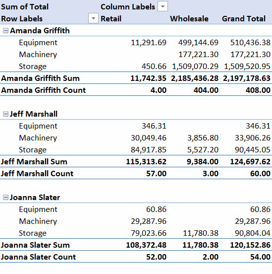
Task: Create and format a pivot table “Sales by seller”

Go to the Sales table and create a new pivot table so that you can view the totals data by seller, product group and sales method.

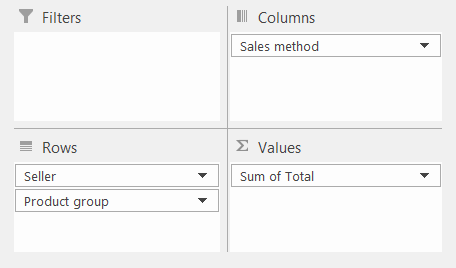
Set a thousands separator formatting for the value field.

Add a blank line between the groups.

Change the name of the sheet to Sales by seller.

Model:

Task: Add subtotals to the pivot table “Sales by seller”

Add Sum and Count as subtotals to see the total sales in dollars and the number of sales/trades. Model:

Now you have already created two separate pivot tables from the tabke you are dealing with. Next, let's explore what happens when we add multiple records to a value field. Are you ready?