Conditional Formatting
Let's imagine a few situations. You are faced with a large amount of data and want to understand it quickly. You first want to see which rows contain relatively large values and which contain small ones, to get a base feeling of the data.
In another situation, you want to create a report that will be presented in a team meeting. With only 10 minutes allotted for the presentation, you want all participants to gain a basic understanding of the data quickly.
In both situations, it is helpful to visualize cells based on their values. So, for example, for large values, the background of the cell is green, and for small values, red.
In Excel, Conditional Formatting works great for this type of formatting. It means formatting that is automatically applied if the value in the cell meets a condition you define.
Conditional formats also allow you to illustrate numbers as data bars, icon sets, or color scales. Excel also has plenty of pre-made conditional formatting options that you can modify. You can also create your own. Conditional formatting can also be used for PivotTables. (PivotTables are introduced in a later chapter of the course, Data Analysis.)
Next, we will delve into how you can get the most out of conditional formatting. As always, you get to learn about the feature yourself in practice, so pick up the exercise workbook and its sheet CONDITIONAL FORMATTING.
The Objective
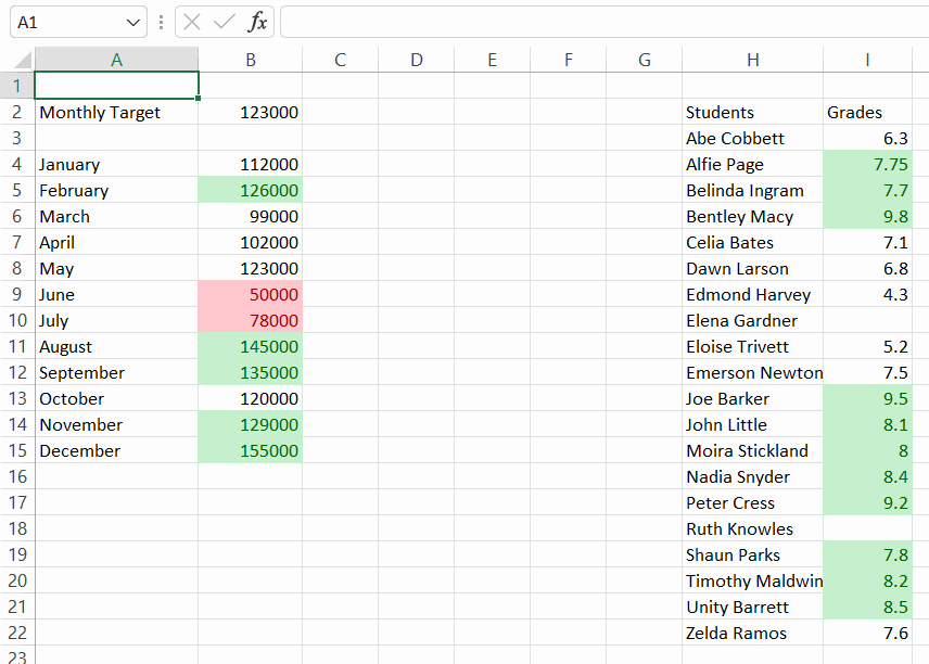
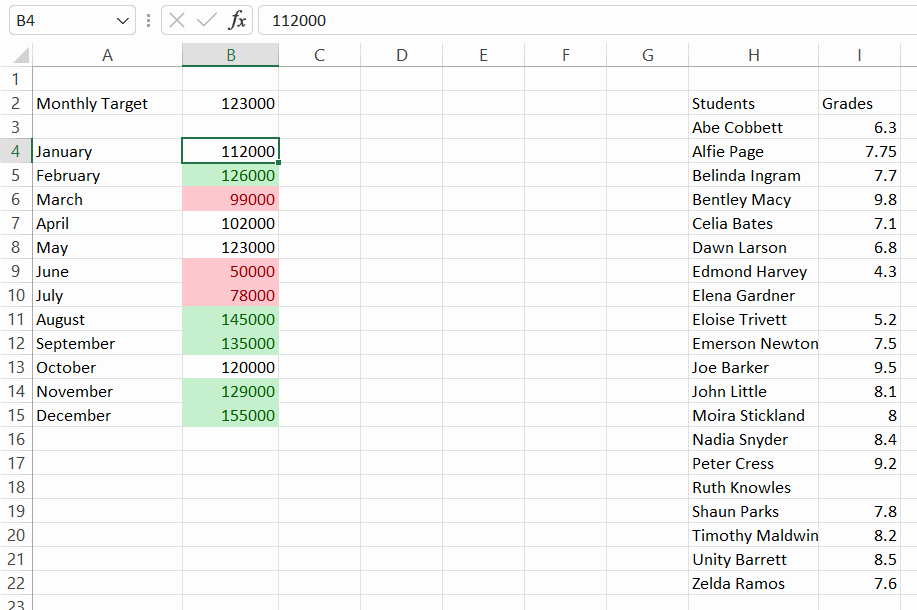
In the task, conditional formatting is applied on the sheet CONDITIONAL FORMATTING of the workbook. This highlights the cells with different colors. Of the sales figures, those that exceed the monthly target in cell B2 are highlighted in green. Values less than 100,000 are highlighted in red.
As an additional task, the red highlighting limit is changed to 90,000, and conditional formatting is added to the values, where values that exceed the average are highlighted using a function.
Video
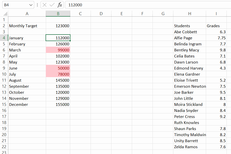
Task: Highlight the cells with less than 100,000 value with red
Do the exercise on the worksheet CONDITIONAL FORMATTING.
Cells that are smaller than 100,000 are highlighted in the sales figures.
Example:
Task: Highlight the cell values larger than the monthly goal in the cell **B2**
Do the exercise on the worksheet CONDITIONAL FORMATTING.
We will set the value used as the limit in a separate cell. In this case, it is visible and can be changed if necessary.
Highlight the numbers greater than the monthly goal, i.e. cell B2, with green.
Example:
Extra Task: Change the minimun limit for conditional formatting to 90,000
Sometimes it's tricky to figure out what kind of conditional formatting a spreadsheet has. Similarly, it is not obvious in the user interface how formatting can be edited. Next, let's look at how we can browse and change formats.
Change the Less Than… conditional formatting limit you applied earlier to 90,000.
Extra Task: Apply conditional formatting based on a formula
Apply conditional formatting, which highlights the values larger than average. We will use the <ek-term id="func_avg" /> function for this.
Model:
You are now at the end of the page. How did you like the exercises? Is there anything you should recapitulate? Remember to take short breaks during your studies! When you're done, you can move on to the next cpagehapter, which is about mixed references.
Does your workbook look like the one below? Are you ready to move on?