Page 2 / 9

Entering Data and Data Types

On this page, you download the Excel practice workbook and start filling it out. You are supposed to use the practice workbook to complete the exercises throughout Basics of Spreadsheets. For starters, you get to try your hand at entering, editing, and deleting data. You will also learn the data formats used in Excel. Try to do all the tasks on the page in one sitting and set aside at least half an hour for the exercise. However, work through the chapter at your own pace: Learning new things is allowed to take some time. From the Excel practice workbook, select the first tab called Input of data.

Download the template file

Download the Excel_1_Exercise.xlsx workbook for yourself. You will do the entire Basics of Spreadsheets in this workbook. Open the file and save it to your chosen location, where you can find it later. If necessary, you can recapitulate the details related to saving on the Saving page.

When you start working on the downloaded file, Excel (or Word, etc.) may open the file in a protected view. In this case, click on the Enable Editing button that appears.

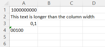
Excel_1_Exercise.xlsxXLSX · Excel_1_Exercise.xlsx

The Objective

In this chapter, we will be working on the Input of data sheet. Afterwards, it should look something like this:

Mallissa on luku '1 000 000 000', leveää tekstiä, luku '0,1' ja luku '00100'

Task: Choose the right sheet

After you open the Excel file, you can see the sheets it contains in the lower corner of the window. You can navigate between the sheets by clicking on their tabs. Start working through the exercises of this chapter from the Input of data sheet.

Task: Enter the data

Do the exercise in the Input of data sheet.

Task: Undoing the data entry

Continue working on the Input of data sheet.

Task: Undo confirmed data

Continue working on the Input of data sheet.

Now remove already entered data.

Task: Editing and replacing old data

If information has already been entered into a cell, you can edit it or replace it with entirely new data.

Continue the task in the sheet Input of data.

Now change the number 150 by clicking on the cell. Enter the number 1000 over the old data and confirm by pressing Enter.

Task: Replace the old value with a lot bigger one

Continue working on the Input of data* sheet.

Replace the value in the A1 cell (1,000) with one billion (1,000,000,000). See how the width of the cell increased?

Info: About file formats

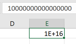
The data entered into a cell can be text, a number, or a formula: We are talking about different data formats. You already entered a number value into a workbook cell earlier, so it should be familiar. Now type in a number consisting of digit one (1) and eighteen zeros in one of the empty cells. See how the number aligns to the right end of the cell, and when the data is wider than the cell, either the column width increases or the number turns to an exponentian number format. The formula bar shows the unformatted value of the cell. Finally, delete the number you entered with the Undo button.

Kaavariville on syötetty liian iso luku, jolloin solussa näkyy luvun eksponenttimuotoilu

Info: What do you mean by exponential format?

The exponential format, also called scientific or engineering notation, for numbers is a compact way to display values in the same column, even when they vary greatly in size. The value after E+ tells you how large the number is, and the value after E- tells you how small it is instead. It's easiest to show you an example:

1.31E+5 is 131,000

1.31E-5 is 0.0000131

One way to think about it is that E+5 is 100,000 (one, and five zeros) and 1.31E+5 is the product 1.31 × 100,000 = 131,000. Using the same logic, you could think that E+3 is 1,000 (three zeros) so 1.31E+3 is 1,310.

On the other hand, you could think that E-5 is 0.00001, so the numerical value tells you the number of zeros before the one. So this way 1.31E-5 is 1.31 × 0.00001 = 0.0000131.

Task: Entering text into a cell

Task: Edit the number format of the cell

Info: Regional and language settings

When you enter data containing numbers, the function settings in Excel determine the format in which the data must be entered and the form in which it's displayed. The default values for these settings depend on the regional and language settings in your Windows.

	#### US settings	#### Finnish settings
#### Decimal separator	`.` (period)	`,` (comma)
#### Thousands separator	`,` (comma)	space
#### Date	month/day/year	day.month.year
#### KeTime of day	hours:minutes AM or PM	hours:minutes
#### Currency symbol	`$`	`€`

When text is entered into a cell, Excel recognizes inputs containing many types of numbers as data of a certain type, such as dates or currency. This affects their formatting. The internal representation is then a number and the related formatting representation. If you select General as the format, the internal representation will be displayed.

Here are some examples:

#### Entered value	#### Formatting	#### Internal representation
10%	Percentage	0.1
7/2/2020	Date	44014 (the amount of days since the beginning of the year 1900)

Info: Half quotation mark vs accent mark

The difference between a half quotation mark (apostrophe) and an accent mark significantly impacts how Excel processes cell content. It's important to understand this distinction to avoid errors and ensure that data is presented correctly. The example images highlight both marks for clarity.

Task: Enter a postal code as text

Sometimes Excel interprets the data as a different type than what is intended.

For example, if you enter data that starts with zero, such as a postal code or phone number that starts with zero, Excel interprets it as a value but automatically formats it so that the leading zeros are omitted.

In this case, the information can be entered as text, wherein the leading zero is included, or the number can be formatted so that the leading zeros are included.

Now let's try entering the postal code as text.

Task: Acknowledge the warning from Excel

It is possible that Excel will warn you about the postal code you have entered. Excel is concerned that you have saved the number as text and issues a warning about it. You will notice this by the small yellow warning triangle that appears next to the data you entered.

Guide

Other various warnings

When using Excel, you may encounter similar warnings in other situations as well.

For example:

Excel will notify you that your formula refers to a cell that is empty. This might mean that you have forgotten to enter data or that your formula is incorrect.
The formula refers to itself either directly or indirectly. Excel warns you about this because such a reference can cause calculation errors or infinite loops.
If Excel does not recognize a formula, it will display an error message such as #DIV/0! (division by zero), #VALUE! (wrong type of value), or #REF! (reference to an invalid cell).
When you try to enter data into a cell with a specific data type (such as date or currency formatting) and the value you enter is not compatible, Excel will issue a warning.
If you try to edit a protected sheet or cell, Excel will display a warning that editing is not allowed.

Info: A hyphen

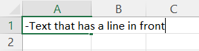
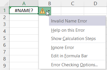
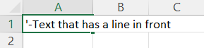
You can also use the apostrophe when you want to add a hyphen (-) in front of the data. Excel assumes that in situations like this, the hyphen is a minus sign which begins a numerical formula.

#### Entering the text

Kuvassa soluun on syötetty '-Tekstiä, jonka edessä on viiva'

#### An error

#### The solution

Tilanne ratkaistaan syöttämällä soluun ''-Tekstiä, jonka edessä on viiva' eli syöttämällä tekstin ja viivan eteen heittomerkki

Info: Formatting a value as ZIP code

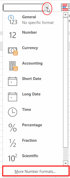
Numero-ryhmän ylhäällä olevaa väkästä napsauttamalla saadaan auki pudotusvalikko

You can also format a value as ZIP code.

If a value is formatted or entered as text (an apostrophe in the beginning), ZIP codes are sorted as text (00100, 01000, 00200, 02000, etc.).

When formatting a value into a ZIP code, it stays as a numerical value. When numerical values are sorted, they will appear in order of magnitude. (00100, 00200, 01000, 02000 etc.)

Open the menu in the Number group on the Home tab, and choose More Number Formats at the end of the opened list.

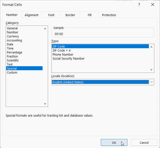
Then follow this path: Special - ZIP Code - OK.

Valitse Luokka Erikoismuotoilu ja sitten oikealta Laji Postinumero

Accessibility and Excel

Accessibility

A recommendation: Name the files in a descriptive way

Excel also has accessibility issues, partly the same as Word, for example, issues around the use of colors. However, here are some simple principles specifically for Excel:

Give the Excel file (workbook) a descriptive name, even if it is rather long. "Data.xls" is a bad name, "Sales statistics 2021.xls" is better.
Name the Excel spreadsheets in a way that describes the content. For example, "Sales" or "Personnel" is better than the default name "Sheet1".
Try to use descriptive headings for the columns, for example, "Name", "Address," and "Personal identification number". This is helpful when, for example, a screen reader user listens to a list of sheets or a description of the information at a certain point of a sheet.

Accessibility checks

Like in Word, also in Excel, on the Review tab you can find the Accessibility group with the function to check the accessibility of the workbook. It will detect problems in the use of colors (lack of contrast), missing alternative texts for graphic objects, and problems that merged cells cause.

“Like playing Battleship.”

For a screen reader user, using an Excel file is difficult because they cannot see where a row or a column ends, and Excel does not tell them. Ending a row or a column is recognized by only empty cells appearing after it. For this reason, avoid empty cells in the middle of a row is. It is better to indicate the absence of information with suitable markings, such as "0" or "–".

Use simple spreadsheets. Avoid writing many different kinds and differently formatted information on the same sheet. Start the data in cell A1, don't leave empty space at the beginning.

A recommendation: Help the reader to figure out the big picture

Not everyone is used to the fact that an Excel file can have many sheets. In addition, it can be challenging to get the big picture, even if the user notices the list of sheets at the bottom of the window. Screen reader programs usually don't even display such a list.

One way to help the reader is to explain, e.g. in an email, what the attached Excel file contains. However, the message and the file are easily separated, or the message is not read properly. That's why it can be a good option for the first sheet to have a description of the contents of the file. It can have, for example, the names of sheets in one column and short descriptions of the content and purpose of the sheet in another. This helps with the problem that the name of a sheet needs to be relatively short and may appear truncated.

A recommendation: Set the first sheet to open first

When Excel saves a file, it also saves information about which sheet is open. This is often useful when editing a file. However, the file recipient may overlook the situation when opening the file. They may think they're at the beginning, while the workbook opens from the middle or even the end. Therefore, before saving the workbook for the last time and closing it, you should open the first sheet.

Now you should be able to enter different information into an Excel workbook. How did the exercises feel? If you feel entering, removing, and editing data in an Excel worksheet is all clear now, click the button below to move on to the next chapter.

Mark as complete: